Relevance of Additive and Nonadditive Genetic Relatedness for Genomic Prediction in Rice Population under Recurrent Selection Breeding
Received: October 14, 2017
Accepted: November 08, 2017
Published: December 18, 2017
Genet.Mol.Res. 16(4): gmr16039849
DOI: 10.4238/gmr16039849
Abstract
In genomic recurrent selection programs of self-pollinated crops, additive genetic effects (breeding values) are effectively relevant for selection of superior progenies as new parents. However, considering additive and nonadditive genetic effects can improve the prediction of genome-enhanced breeding values (GEBV) of progenies, for quantitative traits. In this study, we assessed the magnitude of additive and nonadditive genetic variances for eight key traits in a rice population under recurrent selection, using marker-based relationship matrices. We then assessed the goodness-to-fit, bias, stability and accuracy of prediction for breeding values and total (additive plus nonadditive) genetic values, in five genomic best linear unbiased prediction (GBLUP) models, ignoring or not nonadditive genetic effects. The models were compared using 6174 single nucleotide polymorphisms (SNP) markers from 174 S1:3 progenies evaluated in field yield trial. We found dominance effects accounting for a substantial proportion of the total genetic variance for the key traits in rice, especially for days to flowering. In average of the traits, the component of variance additive, dominance, and epistatic contributed to about 34%, 14% and 9% for phenotypic variance. Additive genomic models, ignoring nonadditive genetic effects, showed better fit to the data and lower bias, in addition to greater stability and accuracy for predict GEBV of progenies. These results improve our understanding of the genetic architecture of the key traits in rice, evaluated in early-generation testing. Clearly, this study highlighted the advantages of additive models using genome-wide information, for genomic prediction applied to recurrent selection in a self-pollinated crop
Introduction
In recurrent selection programs of self-pollinated species, a major challenge is the accurate phenotype prediction of progenies in a synthetic population, for sorting new parents for the next selection cycle. For the achievement of genetic gains, through accumulation of favorable alleles and consequent displacement of the population mean to a desired direction, the prediction must act on the additive effects, i.e., on allelic substitution effects (Bernardo 2010). The additive values or breeding values (BV) becomes relevant in this context, because the gametes and not the genotypes pass from one generation to the next (Hallauer et al. 2010). Therefore, an accurate prediction of genomic-enhanced breeding values (GEBV) of progenies for quantitative traits, is essential to increase the efficient of genomic recurrent selection programs.
Prediction of progeny performance in recurrent selection schemes (i.e., based on phenotypes of progeny testing only) is usually based on genotypic value (i.e., best unbiased linear prediction (BLUP) values or even adjusted means without shrinkage towards the mean, which includes additive and nonadditive genetic effects), estimated without any genetic relationship information (Hallauer et al. 2010). Non-additive genetic effects result from allelic interactions, being the intralocus interaction known as dominance, and interlocus interactions known as epistasis (Lynch and Walsh 1998). Therefore, when nonadditive genetic effects are an important source of variation in trait expression, genotypic selection may induce to recombine progenies that do not have the highest BV. However, when pedigree data is available, expected genetic relationships can be used to obtain BLUP values (Henderson 1975) of BV, by standard pedigree-based models (PBLUP). However, pedigree information is little used in recurrent selection in this purpose, due to the low robustness (small number of selection cycles and progenies involved, besides annotation errors), in addition to not allowing to capitalize the Mendelian segregation – deviations from the expected parents’ contribution (Lynch and Walsh 1998; Hill 2010).
A large number of single nucleotide polymorphisms (SNP markers), widely distributed in the genome, whether in animal or plant species, has been used for genomic prediction (Meuwissen et al. 2001; Bernardo 2010). In addition, marker-based relationship matrices, for additive and nonadditive effects, are feasible to use in genomic prediction (VanRaden 2008; Su et al. 2012). By fitting GBLUP model it is possible to capitalize additive and nonadditive variances between progenies and predict GEBV or total genomic predicted genetic values (GEGV, additive plus nonadditive effects), more accurately than PBLUP model (Su et al. 2012; Muñoz et al. 2014). This is because of the higher accuracy achieved using marker-based relationships than the pedigree-based one, either by the accounting the Mendelian segregation, or even a better decomposition of genetic variance into additive and nonadditive components (Hill 2010). Therefore, in genomic recurrent selection, although the interest is on GEBV of progenies, the consideration of nonadditive effects in GBLUP models may contribute to more accurate and stable genomic predictions (Su et al. 2012; Muñoz et al. 2014; Kumar et al. 2015).
GBLUP models fitted with markers-based relationships matrices are very useful to predict GEBV, in addition to decompose the genetic variance into additive and nonadditive components more precisely. This procedure is useful to better understanding the genetic architecture of complex traits (Muñoz et al. 2014). For an effective decomposition, the terms of these components must be approximately orthogonal, i.e., should assume a clear determination (separation) of components by the implementation of independent terms in the model (Cockerham 1954; Gianola and de los Campos 2008; Hill 2010). In complex pedigree structures, commonly available, this condition is hardly satisfied (Lynch and Walsh 1998; Hill 2010). Moreover, marker-based relationship matrices show less confounding of these variance components, thus allowing a better partitioning of the genetic variance (Muñoz et al. 2014; Bouvet et al. 2015). GEBV are assumed mostly to reflect the allele substitution effects, i.e., additive effects, being that the residual genetic effect therefore can capture nonadditive effects. In inbred lines, the nonadditive effect will represent epistatic interaction effects. However, in noninbred lines (S1, S2 or S3 progenies), other nonadditive effects will include dominance, covariance between additive and dominance effects, epistatic effects and inbreeding depression (Hallauer et al. 2010).
A better understanding of genetic architecture, especially regarding the magnitude of genetic control manifested in the expression of quantitative traits, is also very important for planning actions, especially for the implementation of new selection schemes, aiming to maximize genetic gains (Bernardo 2010). Accounting for dominance and epistatic effects, in addition to additive effects, may not only improve our understanding of the genetic architecture of quantitative traits, but also improve the prediction of phenotypes (Su et al. 2012; Muñoz et al. 2014). This importance arises from the influence of the genetic control of the traits on the efficiency of the schemes used, either in phenotypic or genomic selection approach. Therefore, as the studies of this nature are recent for annual self-pollinated species as rice, more studies are necessary to better understanding the relevance of additive and nonadditive genetic effects of different traits, in genomic prediction models.
In this context, the objectives of this study were i) to assess the magnitude of additive and nonadditive (dominance and epistasis) genetic variances via decomposition of genetic variance using marker-based relationship matrices, for eight quantitative traits in a synthetic population of rice under recurrent selection breeding; and ii) to assess the relevance of additive and nonadditive genetic effects on the goodness-to-fit, bias, stability and predictive accuracy in five GBLUP models, with additive effects and ignoring or not nonadditive effects.
Materials and Methods
Phenotypic data
We used a synthetic population (CNA12S) of irrigated rice, developed at Embrapa, Brazil, in 2002, for recurrent selection breeding. This genetically broad-base population (synthesized with 16 divergent parents) is characterized by its stable resistance to the blast rice (Magnaporthe oryzae B. Couch.). In 2001, crosses were made using 10 elite inbred lines (female parents) and six sources of blast resistance (male parents). Each resistance source participated in three crosses with other elite inbred lines in a factorial mating design, resulting in 18 crosses. F1 plants were backcrossed with the elite parent to result in 18 BC1F1 crosses, constituting subpopulations. After, BC1F1 plants from each subpopulation were crossed with plants from two other subpopulations, resulting in the CNA12S population. Information on the genealogy, development schedule and constituent crosses (subpopulations) are detailed by Morais Júnior et al. (2017a).
The phenotypic evaluation of the population was carried out in a progeny yield trial, performed in the third recurrent selection cycle, conducted in 2015, in Goianira, Goiás (16º 26' 12'' S; 49º 23' 39'' W; 729 m asl). The experimental design was augmented square lattice design, with common check cultivars between blocks 14×17 and two replications, with accommodation of S1:3 progenies and four check cultivars (IRGA 417, BRS 7 Taim, IRGA 424 and BRS Pampa). The first two checks were allocated randomly in all blocks and the other two, alternated, to compose three check cultivars per block. The experimental plots consisted of four 5-m-long rows, spaced 0.17m, with a density of sixty seeds per meter, mechanically sown.
The yield trial was conducted in a lowland area with continuous flooding until grain maturity. Fertilizer was applied in the planting furrow. Weeds and pests were controlled via mechanized spraying. No fungicides were applied, for disease resistance expression. Eight traits were evaluated: incidence of panicle blast – Magnaporthe oryzae (IPB, score), based on a diagrammatic scale (0: no incidence, 1: 1-5%, 3: 6-12%; 5: 13-25%, 7: 26-50%, and 9: more than 50% of infected panicles), according to IRRI (1996); severity of brown spot – Bipolaris oryzae (SBS, score), based on a diagrammatic scale (0.5; 6; 12; 18; 24; 32; and 36% of the leaf area with symptoms), according to Schwanck and Del Ponte (2014); plant height (PH, cm), an average of six measures from ground level to panicle tip, in pre-maturity stage; days to flowering (DTF, days), from sowing to 50% of plants at anthesis; grain yield (GY, kg ha-1) from a 1.36 m2 area at 13% moisture; whole-grain yield (WGY, g), grain mass after mill, according to Crusciol et al. (1999); length-width ratio (LWR); and white and chalky grains (WCG, %). The last two traits were measured using a grain statistical analyzer, model S21®.
Genomic data
From the total of 196 S1:3 progenies, 174 progenies were genotyped. A pooled leaf tissue of eight plants in each progeny was used to obtain purified genomic DNA. DNA extraction was performed according to a commercial kit (Axygen® Inc., USA). Genotyping was performed on Diversity Arrays Technology Pty Ltd (DArT P/L), Canberra, Australia, using DArTseq technology in an Illumina HiSeq 2500® sequencer. A total of 7735 high-quality SNP markers was generated. After quality control (filtering polymorphic markers with call rate higher than 75% and minor allele frequency higher than 5%), 6174 SNP were retained for further genetic analyses.
Missing values (about 4.5% of the data) were replaced by the marker expected values based on the allele frequencies (Pérez-Rodríguez and de los Campos 2014).
Relationship matrices
We calculated additive (Ga) and dominance (Gd) relationship matrices using the SNP marker data. In the calculation of the matrix Ga, we considered the method of VanRaden (2008):
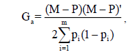
where M is a matrix n x m (n: number of progenies, and m: number of SNP), which specify the genotype of the SNP in each locus; and P is the matrix of observed frequency of the allele i (pi) expressed as 2(pi – 0,5). SNP marker data was converted to the dosage format (-1 for reference-allele homozygotes, 0 for heterozygotes and +1 for alternative-allele homozygotes).
In the calculation of the dominance relationship matrix (Gd), we used the method of Su et al. (2012):

where S is a matrix n x m (n: number of progenies, and m: number of SNP), which specify the SNP-genotype in each locus (ski = 0 - 2piqi if the progeny k is homozygote to the locus i; and ski = 1 - 2piqi if the progeny k is heterozygote to the locus i).
Finally, we generate relationship matrices that captured epistasis of first order, taking the Hadamard product (element-by-element multiplication; denoted #) of matrices (Cockerham 1954; Gianola and de los Campos 2008). Through this procedure, we calculated the following epistatic relationship matrices: (i) additive by additive epistatic interactions (Ga#a ≈ Ga#Ga); (i) dominance by dominance epistatic interactions (Gd#d ≈ Gd#Gd); and (iii) additive by dominance epistatic interactions (Ga#d ≈ Ga#Gd).
Phenotypic data analysis
Single-trait Bayesian analyses were performed to fit the phenotypic data, according to following the linear mixed model: y = Xβ + Z1b + Z2p + e , where y is the vector of observed phenotypic values; β is the vector of fixed effects (i.e., intercept, replication, genotype group – one group of check cultivars and another group of progenies, and effect of check cultivars); b is the vector of random effects of block within replication; p is the vector of random effects of progenies; e is the vector of residues. The terms X, Z1, and Z1 are respective design matrices.
To generate random samples from a joint posterior distribution over the data (y), we used the Gibbs sampling algorithm, allowing obtaining approximate posterior marginal distributions for each parameter. Aiming to consider vague information on the parameters, we considered non-informative improper priors, uniform in the interval [0 → ∞], that lead to proper posterior probabilities, because of the adequate information from the data (y). We assumed normal distributions for the location parameters of fixed and random effects. For variance components, we assumed inverse-Wishart (IW) distributions. The density function of Wishart describes the distribution of the sums of squares and cross products of random effects with normal distribution (Sorensen and Gianola 2007). Therefore, in case of single-trait model, the inverse-Wishart distribution is reduced to a scaled inverse chi-square distribution.
Based on these assumptions on the distributions, we defined the fixed effect priors as normally distributed with expected value (mean) zero and 108 as the degree of belief (variance), for fixing it in the prior at some (large) value. For the variance components associated to random effects, the hyperparameters degree of belief (v) and scale (S) generate a noninformative inverse Wishart distribution by setting v = – 2 and S = 0 (Sorensen and Gianola 2007). Therefore, defining such noninformative priors, the posterior marginal distributions to each parameter given the data (y) are equivalent to those of the REML (restricted maximum likelihood) procedure, in obtaining components of variance, and the BLUP method in the prediction of the random effects.
In the Gibbs sampling setting, using the package ‘MCMCglmm’ in the R platform (R Core Team 2016), a total chain length of 210,000 was used. A burn-in period of 10,000, and thinning of every 20th iteration was used, with a total sample size of 10,000 stored iterations per chain. Conversion was assessed by checking in the chain, and its convergence was assessed by Geweke’s convergence diagnostic. In each chain, we analyzed the posterior mean and the 95% highest posterior density (HPD) interval, for each parameter given the data (y).
Definition of GBLUP models
In this study, we used a sequence of five GBLUP models, according to Muñoz et al. (2014), regarding different marker-based relationship matrices, with additive effects, and ignoring or not nonadditive effects. For each trait, we fitted the following models: additive model (A), which includes only matrix Ga; additive-dominant model (AD), which includes the matrices Ga and Gd; and additive-dominant-epistatic models, model A#A, which includes the matrices Ga, Gd and Ga#a, model D#D, which includes the matrices Ga, Gd and Gd#d, model A#D, which includes the matrices Ga, Gd and Ga#d. Detailed information about this approach is found in the literature ( Su et al. 2012; Muñoz et al. 2014).
We fitted the models using functions of the ‘BGLR’ package of the R platform (R Core Team, 2016). For each model, noninformative prior were defined as a df = 0.1 and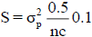 for the degrees of freedom (df) and scale (S) hiperparameters of the scaled-inverse Chi-square (X2) distribution (density
 is given by S./(df – 2), where
 is the phenotypic variance component; and nc is the number of covariance structures (relationship matrices) defined in each model, equal to 1, 2 or 3, for additive-dominant, additivedominant and epistatic-additive models, respectively. In all cases, inferences and predictions were based on a total chain length of 55,000 iterations, after previous analyses of some MCMC chains. A burn-in period of 5,000, and thinning every 5th iteration was used, resulting in a total sample size of 10,000 stored iterations per chain. Details about priori definitions in functions of the 'BGLR' package are presented by Pérez-Rodriguez and
de los Campos (2014).
is the phenotypic variance component; and nc is the number of covariance structures (relationship matrices) defined in each model, equal to 1, 2 or 3, for additive-dominant, additivedominant and epistatic-additive models, respectively. In all cases, inferences and predictions were based on a total chain length of 55,000 iterations, after previous analyses of some MCMC chains. A burn-in period of 5,000, and thinning every 5th iteration was used, resulting in a total sample size of 10,000 stored iterations per chain. Details about priori definitions in functions of the 'BGLR' package are presented by Pérez-Rodriguez and
de los Campos (2014).
We obtained the following components of genetic variance for each model and trait: narrow-sense (h2) and broad-sense (H2) heritability, as the ratio of additive () to phenotypic variance ( sum of all variance components in the model), and the ratio of total genetic variance 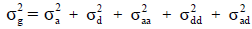 to phenotypic variance, respectively, the dominance to total variance ratio as
  the epistatic to total variance ratio as
  These variance components varied according to the model. For each component of genetic variance, we obtained the posterior mean and respective standard error (SE) of the mean, using a cross-validation procedure.
Comparison of models and cross-validation procedure
GBLUP models were compared using the Akaike’s Information Criterion (AIC; Akaike 1974), defined by the expression  where k = number of parameters estimated, and
 is the maximized value of the likelihood function for the model. Therefore, AIC combines a measure of model fit (maximum of the likelihood) with a measure of model complexity (number of estimated parameters) over all iterations after burnin. The model with lowest AIC is chosen as the best fitting model. To quantify the relative likelihood of the models, i.e., the probability that the ith model minimizes the (estimated) information loss, we employed the expression exp((AICmin − AICi)/2), where exp is the exponential function, and AICmin is the AIC with lowest value.
For each trait, ability and stability of the models in the prediction of breeding values (BV) or total genetic values (GV) were also evaluated. We calculated the Pearson's correlation between BVf or GVf and the estimated genotypic value (BLUP, Yf) of progenies from the full dataset (without cross-validation), as a measure of model’s predictive ability. The model’s predictive stability was calculated via Pearson's correlation between BVfor GVf of progenies from the full dataset (without cross-validation) and BVv or GVv of progenies from the validation dataset (with cross-validation), respectively. For each model and trait, we also calculated the mean square error (MSE) between BVf and BVv, and between GVf and GVv. In addition, for each model and trait, Yv values were linearly regressed on BVv or GVv of progenies from the validation set, where the slope coefficient is defined as a measurement of the degree of bias of a model. In this context, unbiased models are expected to have a slope coefficient of one.
Averaged predictive accuracy of each model and trait was computed by Pearson's correlation between breeding values (BVv) or total genetic values (GVv) and estimated genotypic value (Yv) of the validation dataset. For this procedure, we used the cross-validation scheme TRN-TST partitions (Pérez-Rodríguez and de los Campos 2014), with 50 TRN-TST random partitions of the total dataset (N), considering 90% for training (TRN) and 10% for validation or testing (TST). Specifically, this scheme corresponds to a 10-folk cross-validation with 50 random partitions (replications of the original k-folk procedure) of the total dataset, aiming to raise the precision of the estimate of accuracy. We also estimated the standard error (SE) of the mean of each parameter obtained through cross-validation (predictive stability, slope coefficient and predictive accuracy).
Results
Population characterization
Regarding the population structure based on the additive relationship matrix, on observing the dispersion of the progenies in the space of the first two principal components (Figure 1), no prominent structure was found associated to the progenies or subpopulations. The eighteen subpopulations (S01 to S18) constituents of the CNA12S population presented great overlapping, i.e., there was a high sharing of alleles between them. Therefore, this result does not justify the need to perform stratified sampling in this population, or even any analysis that considers dependence of the allele effects between possible clusters, for genomic prediction.

Figure 1: Dispersion of S1:3 progenies of the CNA12S population (identification of 18 constituent subpopulations – S01 to S18), in relation to the first (PC1) and second (PC2) principal components, estimated in relation to the additive relationship (Ga).
Estimates of parameters related to experimental precision and genetic variability, associated with the traits evaluated in the S1:3 progenies from the third recurrent selection cycle of this population, were presented by Morais Júnior et al. (2017a). For all the traits, were observed considerable genetic variability and high experimental precision associated with the phenotypic data, therefore, with high potential for fitting accurate genome-enabled prediction models. In addition, overall empirical distribution of the phenotypic data of genotypes (progenies and check cultivars) for each trait were approximately normal (data not shown), which justifies the use of Gaussian models, either to obtain genotypic values (Y, BLUP related to the genotypic effects) or even for application of genomic prediction.
Proportion of additive and non-additive variance components
Proportions of components of genetic variance derived from the decomposition of the phenotypic variance for each GBLUP model and trait are presented in Figure 2. As expected, the narrow-sense (h2) was lower than the broad-sense heritability (H2), for all prediction models and traits. Narrow-sense heritability (h2) estimated via additive model (A) decreased after including nonadditive (dominance and epistatic) effects in additive-dominance (AD) or additive-dominance-epistatic (A#A, D#D, A#D) models, for all traits. Across all traits, the decrease in h2 was 18% when dominance effects were accounted for (i.e., using AD instead of A), and 26% when dominance and epistatic effects were accounted for (i.e., using A#A, D#D and A#D instead of A). The highest decrease in h2 was observed for DTF (59% in average, using AD, A#A, D#D and A#D instead of A), and the smallest for WCG (8% in average, using AD, A#A, D#D and A#D instead of A). Specifically, when the dominance effects were assumed to be absent, using the additive model (A), h2 ranged from 0.22 (for DTF) to 0.66 (for WCG). This result is explained by some dependence between additive and nonadditive matrices, which is not able to effectively explain independently the corresponding genetic effects. Considering the dominance effect, in the model AD, h2 reduced about 18% in average; with a variation of 0.08 (for DTF) to 0.38 (for WCG). Therefore, these results reflect a substantial amount of dominance variance (d2) for most of the traits.

Figure 2: Posterior mean to the proportion of genetic variance components from the partitioning of broad-sense heritability (H2): additive variance (h2), dominance variance (d2) and epistasis variance (i2), for each model. The traits are: grain yield (GY, kg ha-1), plant height (PH, cm), days to flowering (DTF, days), incidence of panicle blast (IPB, score), severity of brown spot (SBS, score), whole-grain yield (WGY, g), length-width ratio (LWR), and white and chalky grains (WCG, %). All proportion values were significant based on the SE estimates.
The additive-dominant model (AD) was extended to include additive-by-additive (A#A), dominant-by-dominant (D#D) and additive-by-dominant (A#D) first-order epistatic interaction effects (Figure 2). When comparing the three additive-dominance-epistatic models, small-to-moderate alterations in the proportion of the genetic components were observed to each trait, although occurring strong changes between traits. When epistasis effects were considered, the components h2 and d2 reduced about 9% and 13% compared to the model AD, in the average of all traits. The proportion of epistasis variance (i2) was 0.07 (for A#A), 0.10 (for D#D) and 0.10 (for A#D). In the average of these models, i2 ranged from 0.05 (for SBS) to 0.18 (for WGY), reflecting the smaller contribution of this component than to d2, for the most traits. In the average of all traits, the components h2, d2 and i2 contributed with about 34%, 14% and 9% for phenotypic variance.
Model goodness-of-fit, ability, stability and predictive accuracy
The goodness-of-fit of the models was estimated using the full dataset, i.e., without cross-validation (Table 1). As the predictive ability, correlations between breeding values (BV) and genotypic values (Y) were lower that the correlations between total genetic value (GV) and Y, for all traits. The correlations between BVf and Yf ranged from 0.85 (for DTF) to 0.97 (for WCG), smaller than the correlations between GVf and Yf, that ranged from 0.90 (for DTF) to 0.98 (for WCG), with marked differences between models, for most traits. The largest differences between the BV and GV predictive ability were detected for DTF, and the smallest for WCG, reflecting the best and worse fit to the genotypic values, respectively, by considering the nonadditive (dominance and epistatic) effects in models. A slight decrease in the differences of BV predictive ability and slight increase in the differences of GV predictive ability, between the models, were observed when nonadditive effects were considered.
| Trait | Model | Predictive ability | LogLb | AICb | L( θ )b | |
|---|---|---|---|---|---|---|
| r(BVf, Yf)a | r(GVf, Yf)a | |||||
| GY | A | 0.89 | - | -1164.3 | 2441.0 | 1.00 |
| AD | 0.89 | 0.91 | -1160.0 | 2443.0 | 0.38 | |
| A#A | 0.88 | 0.93 | -1153.6 | 2443.4 | 0.31 | |
| D#D | 0.88 | 0.93 | -1154.8 | 2443.0 | 0.37 | |
| A#D | 0.88 | 0.93 | -1152.6 | 2442.1 | 0.58 | |
| A | 0.92 | - | -391.7 | 915.6 | 1.00 | |
| AD | 0.92 | 0.94 | -385.1 | 915.7 | 0.94 | |
| PH | A#A | 0.91 | 0.95 | -381.4 | 917.1 | 0.47 |
| D#D | 0.91 | 0.95 | -381.5 | 916.1 | 0.78 | |
| A#D | 0.91 | 0.95 | -381.5 | 916.3 | 0.69 | |
| A | 0.78 | - | -371.5 | 810.5 | 1.00 | |
| AD | 0.76 | 0.90 | -351.8 | 812.3 | 0.40 | |
| DTF | A#A | 0.76 | 0.93 | -346.5 | 814.1 | 0.17 |
| D#D | 0.76 | 0.93 | -346.7 | 813.1 | 0.28 | |
| A#D | 0.76 | 0.93 | -346.6 | 813.6 | 0.21 | |
| A | 0.87 | - | -267.6 | 642.5 | 1.00 | |
| AD | 0.87 | 0.90 | -261.5 | 644.6 | 0.36 | |
| IPB | A#A | 0.86 | 0.92 | -254.5 | 645.2 | 0.26 |
| D#D | 0.86 | 0.92 | -256.3 | 645.3 | 0.25 | |
| A#D | 0.86 | 0.92 | -255.6 | 645.5 | 0.23 | |
| A | 0.95 | - | -421.1 | 999.5 | 1.00 | |
| AD | 0.95 | 0.96 | -417.9 | 1000.1 | 0.76 | |
| SBS | A#A | 0.95 | 0.96 | -415.3 | 1001.0 | 0.49 |
| D#D | 0.94 | 0.96 | -414.9 | 1000.1 | 0.76 | |
| A#D | 0.94 | 0.96 | -414.6 | 1000.1 | 0.77 | |
| A | 0.87 | - | -419.5 | 930.1 | 1.00 | |
| AD | 0.86 | 0.91 | -411.5 | 931.3 | 0.55 | |
| WGY | A#A | 0.85 | 0.96 | -395.0 | 931.3 | 0.53 |
| D#D | 0.85 | 0.94 | -400.0 | 932.4 | 0.32 | |
| A#D | 0.85 | 0.97 | -390.2 | 932.1 | 0.37 | |
| A | 0.94 | - | 139.9 | -151.0 | 1.00 | |
| AD | 0.93 | 0.95 | 144.9 | -150.0 | 0.60 | |
| LWR | A#A | 0.91 | 0.97 | 155.6 | -150.7 | 0.84 |
| D#D | 0.93 | 0.96 | 155.6 | -150.7 | 0.84 | |
| A#D | 0.92 | 0.96 | 150.2 | -150.6 | 0.79 | |
| A | 0.97 | - | -415.4 | 1004.1 | 1.00 | |
| AD | 0.97 | 0.97 | -412.8 | 1004.7 | 0.74 | |
| WCG | A#A | 0.95 | 0.98 | -406.0 | 1005.0 | 0.64 |
| D#D | 0.96 | 0.97 | -411.2 | 1005.4 | 0.53 | |
| A#D | 0.96 | 0.98 | -410.0 | 1004.9 | 0.69 | |
Table 1. Posterior mean of predictive ability and parameters related to the goodness-of-fit of the models, for grain yield (GY, kg ha-1), plant height (PH, cm), days to flowering (DTF, days), incidence of panicle blast (IPB, score), severity of brown spot (SBS, score), whole-grain yield (WGY, g), length-width ratio (LWR) and white and chalky grains (WCG, %)
The relative model quality was assessed through an Akaike’s information criterion (AIC) (Table 1). From this criterion, the relative likelihood [L( θ )] of each fitted model was also considered as probability’s measure that the model minimizes the (estimated) information loss, in relation to the model with lowest AIC value. Based on the lowest estimated AIC, the additive model (A) presented a better fit to the data, and consequently the higher relative likelihood [L( θ ) = 1], for all traits. Therefore, the evidence that the best model for all traits include only additive effects is very strong.
estimated from the full dataset. b LogL: log-likelihood function; AIC: Akaike’s Information Criterion; and L( θ ): relative likelihood of the model.
Measures related to predictive stability, mean square error (MSE) and slope regression (b) of each model, to predict breeding or total genetic values of progenies for each trait, are showed in Table 2. The predictive stability measures the dependency of BV or GV values on the phenotype, defined as correlation between BVf or GVf of progenies from the full dataset and BVv or BVv of progenies from the validation dataset. As expected for all traits evaluated, predictive stability was higher to BV prediction, with correlations ranging from 0.65 (for LWR) to 0.85 (for IPB), than to GV prediction, with correlations ranging from 0.46 (for LWR) to 0.82 (for WCG). To each trait, non-significant differences were observed in BV or GV predictive stability between the models.
| Trait | Model | Predictive stability | MSE | Slope coefficient (b) | |||||
|---|---|---|---|---|---|---|---|---|---|
| r(BVf, Yv)a | r(GVf, Yv)a | (BVf, BVv) | (GVf, GVv) | (Yv~ BVv) | (Yv ~ GVv) | ||||
| A | 0.76 ± 0.01 | - | 35845 | - | 1.03 ± 0.04 | - | |||
| AD | 0.76 ± 0.01 | 0.72 ± 0.01 | 31972 | 44295 | 1.12 ± 0.03 | 1.03± 0.04 | |||
| GY | A#A | 0.77 ± 0.01 | 0.68 ± 0.02 | 27120 | 54492 | 1.23 ± 0.02 | 1.05± 0.04 | ||
| D#D | 0.77 ± 0.01 | 0.69 ± 0.02 | 30614 | 52309 | 1.13 ± 0.03 | 1.03± 0.04 | |||
| A#D | 0.77 ± 0.01 | 0.68 ± 0.02 | 27314 | 55392 | 1.24 ± 0.02 | 1.05± 0.03 | |||
| A | 0.80 ± 0.01 | - | 2.78 | - | 0.97 ± 0.06 | - | |||
| AD | 0.81 ± 0.01 | 0.77 ± 0.01 | 2.20 | 3.44 | 1.14 ± 0.05 | 0.97± 0.06 | |||
| PH | A#A | 0.82 ± 0.01 | 0.76 ± 0.01 | 1.80 | 3.81 | 1.28 ± 0.04 | 1.00± 0.06 | ||
| D#D | 0.82 ± 0.01 | 0.76 ± 0.01 | 2.06 | 3.80 | 1.17 ± 0.04 | 0.98± 0.06 | |||
| A#D | 0.82 ± 0.01 | 0.75 ± 0.01 | 1.91 | 3.84 | 1.24 ± 0.04 | 0.99± 0.06 | |||
| A | 0.82 ± 0.01 | - | 0.42 | - | 1.12 ± 0.03 | - | |||
| AD | 0.81 ± 0.01 | 0.68 ± 0.02 | 0.11 | 1.10 | 2.51 ± 0.22 | 0.94± 0.01 | |||
| DTF | A#A | 0.82 ± 0.01 | 0.65 ± 0.02 | 0.07 | 1.34 | 3.13 ± 0.31 | 0.96± 0.01 | ||
| D#D | 0.82 ± 0.01 | 0.64 ± 0.02 | 0.09 | 1.35 | 2.76 ± 0.25 | 1.01± 0.01 | |||
| A#D | 0.82 ± 0.01 | 0.64 ± 0.02 | 0.08 | 1.35 | 2.96 ± 0.28 | 0.99± 0.01 | |||
| A | 0.84 ± 0.01 | - | 0.32 | - | 0.96 ± 0.05 | - | |||
| AD | 0.85 ± 0.01 | 0.81 ± 0.01 | 0.27 | 0.43 | 1.09 ± 0.04 | 0.95± 0.05 | |||
| IPB | A#A | 0.85 ± 0.01 | 0.77 ± 0.01 | 0.22 | 0.54 | 1.22 ± 0.03 | 0.96± 0.05 | ||
| D#D | 0.85 ± 0.01 | 0.78 ± 0.01 | 0.24 | 0.51 | 1.14 ± 0.04 | 0.97± 0.05 | |||
| A#D | 0.85 ± 0.01 | 0.77 ± 0.01 | 0.22 | 0.52 | 1.22 ± 0.03 | 0.97± 0.05 | |||
| A | 0.78 ± 0.01 | - | 6.95 | - | 1.01 ± 0.07 | - | |||
| AD | 0.78 ± 0.01 | 0.76 ± 0.01 | 6.25 | 7.73 | 1.06 ± 0.07 | 1.02± 0.07 | |||
| SBS | A#A | 0.79 ± 0.01 | 0.75 ± 0.01 | 5.77 | 8.39 | 1.11 ± 0.07 | 1.04± 0.07 | ||
| D#D | 0.79 ± 0.01 | 0.75 ± 0.01 | 5.94 | 8.29 | 1.08 ± 0.07 | 1.03± 0.07 | |||
| A#D | 0.79 ± 0.01 | 0.75 ± 0.01 | 5.73 | 8.39 | 1.12 ± 0.07 | 1.04± 0.07 | |||
| A | 0.76 ± 0.01 | - | 1.74 | - | 1.05 ± 0.01 | - | |||
| AD | 0.76 ± 0.01 | 0.70 ± 0.01 | 1.34 | 2.52 | 1.30 ± 0.02 | 1.06± 0.01 | |||
| WGY | A#A | 0.78 ± 0.01 | 0.60 ± 0.02 | 0.54 | 4.09 | 2.15 ± 0.11 | 1.14± 0.02 | ||
| D#D | 0.77 ± 0.01 | 0.64 ± 0.01 | 1.21 | 3.55 | 1.40 ± 0.03 | 1.07 ± 0.01 | |||
| A#D | 0.78 ± 0.01 | 0.59 ± 0.02 | 0.60 | 4.49 | 2.05 ± 0.10 | 1.16 ± 0.02 | |||
| A | 0.72 ± 0.01 | - | 5e10-4 | - | 0.94 ± 0.04 | - | |||
| AD | 0.70 ± 0.02 | 0.46 ± 0.02 | 4e10-4 | 5e10-4 | 1.08 ± 0.02 | 0.93 ± 0.04 | |||
| LWR | A#A | 0.65 ± 0.02 | 0.47 ± 0.02 | 3e10-4 | 6e10-4 | 1.60 ± 0.03 | 1.04 ± 0.03 | ||
| D#D | 0.68 ± 0.02 | 0.46 ± 0.02 | 4e10-4 | 6e10-4 | 1.13 ± 0.01 | 0.95 ± 0.03 | |||
| A#D | 0.67 ± 0.02 | 0.46 ± 0.02 | 4e10-4 | 6e10-4 | 1.33 ± 0.01 | 0.99 ± 0.03 | |||
| A | 0.82 ± 0.01 | - | 10.26 | - | 1.04 ± 0.07 | - | |||
| AD | 0.83 ± 0.01 | 0.82 ± 0.01 | 9.32 | 11.13 | 1.08 ± 0.06 | 1.04 ± 0.07 | |||
| WCG | A#A | 0.85 ± 0.01 | 0.80 ± 0.01 | 6.87 | 12.46 | 1.20 ± 0.06 | 1.10 ± 0.06 | ||
| D#D | 0.83 ± 0.01 | 0.81 ± 0.01 | 8.91 | 11.55 | 1.09 ± 0.06 | 1.05 ± 0.07 | |||
| A#D | 0.84 ± 0.01 | 0.81 ± 0.01 | 8.26 | 11.78 | 1.13 ± 0.06 | 1.07 ± 0.07 | |||
a Posterior mean estimates of Pearson's linear correlation; MSE: mean square error; BVf and GVf : breeding value and total genetic value estimated from the full dataset; BVv, GVv and Yv: breeding value, total genetic value and genotypic value estimated from the validation dataset.
Table 2. Posterior mean of predictive stability, mean square error (MSE) and slope coefficient (b) of the models, for grain yield (GY, kg ha-1), plant height (PH, cm), days to flowering (DTF, days), incidence of panicle blast (IPB, score), severity of brown spot (SBS, score), whole-grain yield (WGY, g), length-width ratio (LWR) and white and chalky grains (WCG,%)
Across models and traits, the mean square error (MSE) for BV prediction presented lower values than obtained for GV prediction (Table 2). For each trait, no marked differences between MSE were observed for GV prediction. As expected, for all traits, additive model (A) based prediction showed the higher MSE, because this model is not able to explain all the genetic variation, thus resulting in remaining variation included into the residual term. A pronounced decrease in the differences of MSE for BV prediction and a prominent increase in the differences of MSE for GV prediction, between the prediction models, was observed when nonadditive effects were included in the models.
As a measure of bias of prediction for each model, we calculated the slope regression of Yv on BVv or GVv ( Table 2). Whereas slope coefficients greater than 1 indicated a biased underestimation in prediction, and values smaller than 1 indicated a biased overestimation, unbiased models are expected to have a slope coefficient of 1. For all traits, except for DTF, slopes of the additive model (A) were not significantly different than 1, indicating no significant bias in BV prediction. When nonadditive effects were included in the models AD, A#A, D#D and A#D, there were significant underestimations in BV prediction, for all traits. For DTF, these underestimations were even more accentuated, with slopes coefficients greater than 2. By the other hand, in GV prediction there were no significant bias, for most of the models and traits. In addition, the additive-dominance-epistatic models showed the larger slopes, with more significant bias, either in BV or GV prediction. The suitability of additive, additive–dominance and additive–dominance-epistatic prediction models was assessed by BV and GV predictive accuracy (Figure 3).

Figure 4: Posterior mean of predictive accuracy of each model, based on prediction of breeding values or total genetic values, for grain yield (GY, kg ha-1), plant height (PH, cm), days to flowering (DTF, days), incidence of panicle blast (IPB, score), severity of brown spot (SBS, score), whole-grain yield (WGY, g), length-width ratio (LWR), and white and chalky grains (WCG, %). The error bars represent standard error of the mean.
Across the models, BV accuracy ranged from 0.31 (for DTF) to 0.68 (for WCG), while GV accuracy ranged from 0.33 (for DTF) to 0.68 (for WCG). As expected, the predictive accuracy is much lower than measures of correlations related to goodness-of-fit (predictive ability and stability), due to considering independent data between training and testing sets, via cross-validation.
Based on the intervals of standard error (SE) of the mean, no clear differences were detected in accuracy between the models, not even between BV and GV accuracy, for each trait. This result can be attributed to the marked variation in the accuracy of all the models, among the 50 random subsets of the cross-validation procedure, thus resulting in overlapping intervals (data not shown). Considering all traits, BV predictive accuracy of the additive model (A) was high correlated (r = 0.94) with the h2 component of the traits (Figure 4). This result expresses the strong influence of the trait heritability on the predictive accuracy.

Figure 4: Relationship (linear regression) between the predictive accuracy of breeding values and the trait narrow-sense heritability (h2) for the additive model (A). Pearson's correlation coefficient (r) equal to 0.94 (p-value < 0.001).
Finally, we also estimated significant correlations of moderate to high magnitude (Table 3), which ranged from 0.32 (additive relationship vs dominance relationship) to 0.86 (dominance relationship vs dominance by dominance epistatic interaction), suggesting that the matrices entries are positively associated.
| Matrixa | Gd | Ga#a | Ga#d | Gd#d |
|---|---|---|---|---|
| Ga | 0.323** | 0.663** | 0.851** | 0.417 ** |
| Gd | - | 0.317** | 0.275** | 0.860 ** |
| Ga#a | - | - | 0.851** | 0.511 ** |
| Ga#d | - | - | - | 0.499 ** |
aSignificance computed by Mantel’s test with 10,000 permutations, where ** p-value < 0.001. Ga: additive relationship; Gd: dominance relationship; Ga#a: additive by additive interaction; Gd#d: dominance by dominance interaction; Ga#d: additive by dominance interaction.
Table 3. Estimates of Pearson’s linear correlation between genetic relationship matrices
Discussion
In the context of a recurrent selection program, the availability of a dense genomic markers panel enables the genotyping of progenies for many SNP markers, thus, obtaining genomic relationship matrices (G-matrix). The application of G-matrices in generating measures of genetic variance parameters from synthetic populations of self-pollinated species has not yet been explored. Therefore, the present study was motivated by the fact that no other study has compared GBLUP models, including simultaneously additive and nonadditive effects, either to investigate the traits genetic architecture, or to genomic prediction in rice. The studies already carried out in rice have exploited and considered only additive effects in the genomic prediction, evaluating different model approaches, based either on parametric or nonparametric methods (Grenier et al. 2015; Onogi et al. 2015; Spindel et al. 2015).
Additive and nonadditive genetic variances
In this study, we fitted GBLUP models to estimate additive and nonadditive genetic variation, in addition to breeding and total genetic values, via G-matrices-based analysis, using genome-wide SNP markers. Therefore, based in marker-based genetic models, this is the first formal attempt to estimate additive, dominance, and epistatic variances of rice phenotypes, especially in a synthetic population (CNA12S) developed for recurrent selection breeding. We decided not to use the pedigree data of this population, since other studies (Muñoz et al. 2014; Kumar et al. 2015; Gamal El-Dien et al. 2016) already have evidenced the lower efficiency of pedigreebased models to capture and explain genetic relatedness. According to these authors, the use of average numerator relationship matrices recognizably producing less realistic estimates of genetic variance, because of limited and biased disentanglement of additive variance from all nonadditive factors through genetic variance decomposition, than using marker-based models (having the capacity to exploit the Mendelian sampling term between progenies).
Our results showed that when additive and nonadditive effects were used together, the variance explained by the additive component decreased. By the other hand, the broad-sense heritability of all traits (sum of the heritabilities due to all genetic effects considered) increased when dominance and epistatic effects were accounted for. One reason to this tendency is that the additive component alone absorbs some nonadditive variance. Thus, this indicates that the relationship matrices are in a “tug-of-war” state over the same variance, as verified in other studies (Su et al. 2012; Muñoz et al. 2014; Bouvet et al. 2015; Lopes et al. 2015; Gamal El- Dien et al. 2016). This can be explained by some nonorthogonality existing in the distribution of additive and nonadditive effects, thus, suggesting dependency between variance components.
The confounding nature of additive and nonadditive effects depends of the distribution of allele frequencies, linkage disequilibrium (LD) patterns, and trait genetic architecture, being that certain proportion of the variance due to interaction of alleles can upwardly biased the estimate of additive variance (Lu et al. 1999; Hill et al. 2008; Zuk et al. 2012). In this sense, for all traits, the additive variance was overestimated when using the additive model (A), being 62% of the overestimated additive variance explained by the dominance variance, and 38% by the epistatic variance, across all traits. Therefore, these results evidence a large fraction of dominance on the total genetic variance, in all rice phenotypes evaluated. This is even more pronounced for DTF, a trait recognizably controlled by expressive effect of dominance in rice (Kawakata and Yajima 1995; Morais Júnior et al. 2017b).
It is worth to highlight that, the genotyping was performed for a pooled DNA of eight plants of each S1:3 progeny, therefore, the estimated genetic variance corresponds to that expected between S1 progenies. It is also necessary to highlight that this population comes from multiple crosses, with unequal contribution of the parents (inbred S1:3 progenies), therefore, with allele frequency ≠ 0.5. In this case, the genetic variance  of the population in generation S1 (equivalent to F3, with inbreeding coefficient = 0.5), omitting epistatic effects, is about:
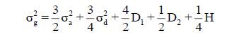
(Cockerham 1963), where  and
and  are the additive and dominance variances; D1 is the covariance between additive effects and homozygous dominance effects; D2 is the variance of homozygous dominance deviations; and H is the sum of homozygous dominance deviations, squared. Therefore, there are ‘hidden’ nonadditive components even if an additive model is fitted. Thus, defining genetic relationship matrices might arises certain overestimation of the components of genetic variance relative to the expected in S1, since other important genetic effects (D1, D2 and H) also explain the phenotypes.
It is known that the application of genomic data to estimate additive, dominance, and epistatic variances allows us to better understand the genetic architecture of traits. Compared to pedigree data, the use of genome-wide markers has been described as a more precise alternative to partition the genetic variance (Vinkhuyzen et al. 2013; Muñoz et al. 2014; Gamal El-Dien et al. 2016). However, it is worth to highlight that genomic estimates may presents its own pitfalls. In this case, the proportion of the variance explained by the markers can be underestimated, because of the non-captured variance, a phenomenon described as “the case of the missing heritability” (Maher 2008). This might happen if the causal variants (genes/QTLs) are not in linkage disequilibrium (LD) with the markers used in the estimation of the variance components. This phenomenon can explain the differences detected in other studies (Vinkhuyzen et al. 2013; Muñoz et al. 2014; Bouvet et al. 2015), between genomic and pedigree based variance components, being that pedigree-based analysis often overestimate additive variance compared to markers-based analysis. However, according to Lopes et al. (2015), despite the considerable differences between variance components, it is still uncertain if such differences are more likely due to an underestimation with genomics or due to an overestimation with pedigree data.
Other pitfall in the genomic data is regarding the estimation of epistatic variance, using relationship coefficients of epistatic variance–covariance matrices defined by Hadamard product, which assumes a population in linkage equilibrium and not linked markers (Schnell 1963). Therefore, synthetic populations always have some LD degree, desirable to genomic prediction, and due to the large amount of SNP markers, some of these can be tightly linked. In this case, the use of Hadamard matrix multiplication should lead to some bias in epistatic variance estimates. According to Schnell (1963), the recombination rate should be taken into account for in the definition of epistatic coefficient matrices. However, the pattern of recombination rate is highly variable across the genome, besides of negative correlation with genome size, in several species, as rice (Tiley and Burleigh 2015), which makes its account a very difficult task. Therefore, using marker-based relationship matrices without this correction, the models cannot be able to clearly estimate the epistatic variance.
Influence of additive and nonadditive effects on models fitting and accuracy
For all traits, the values of AIC and relative likelihood indicate better-fitting of additive model (A). Therefore, as the additive effects are able to capture part of the effects due to dominance and epistasis, as already described, such effects are not expressive when accounted in the prediction model. Our results also revealed that for BV prediction, the ability varied considerably between models, but remained certain higher values for the additive model (A). Therefore, as our interest in rice breeding is on BV prediction, to obtain better-fitted models, the nonadditive effects can be neglected, there being no reason to consider them into genomic-enabled prediction models. Comparisons with other studies should be carried out with caution because the results regarding the prediction are highly dependent of the population generation and the applied method. The results assessed in our study were like those in a Eucalyptus hybrid population (Bouvet et al. 2015), but opposite to those in a Pinus taeda multifamily population (Muñoz et al. 2014), in three purebred pig populations (Lopes et al. 2015), and in a breeding population of cassava (Manihot esculenta) (Wolfe et al. 2016). In these last studies, better fit to models or predictive ability were detected by the inclusion of nonadditive effects, possibly due to larger magnitude of such effects given the structure of families in the population, or even by the used training dataset size.
Aiming to measure the influence of the genotypes to predicted BV, we tested how the inclusion of additive or nonadditive genetic effects affected the prediction stability, comparing the results from the full dataset, with the results from validation set. For all traits, we observed non-significant differences between the models, regarding the stability of the BV prediction. Therefore, the application of nonadditive relationship matrices not contribute to generate models with more stable BV prediction than additive model, although the mean square errors (MSE) of the additive-dominance or additive-dominance-epistatic models decreased noticeably when compared with the additive model, for all traits. Not surprisingly, the significant upwards bias of the BV prediction, with the inclusion of nonadditive effects in the models, also can be an evidence that additive model is enough for genomic prediction in this rice population. This pattern of bias in the prediction may have happened because models with nonadditive effects inflated the predicted BV, promoting a biased underestimation of such effects. These results indicate that, for the evaluated rice phenotypes, a consistent (high stability and low bias) BV prediction can be achieved simply by additive prediction models.
Conclusion
Finally, this study improved our current understanding of the genetic architecture of the main traits evaluated in rice breeding programs, such information should be considered when developing effective breeding schemes of genomic recurrent selection. This study also shows that the nonadditive genetic effects, although being an important source of genetic variation for rice phenotypes, are not relevant for prediction of breeding values of progenies, as new parents for recombination crosses in population of recurrent selection. These results are very important, since only the breeding values are relevant to promote genetic gains between cycles in intrapopulation recurrent selection, being effectively transferred to further generations.
Acknowledgments
The authors dedicate this article to the memory of Dr. Orlando Peixoto de Morais. We thank the entire rice breeding team at Embrapa, especially the research assistants and field workers, and thank Capes/Brazilian Ministry of Education, for granting a scholarship to the first author.
About the Authors
Corresponding Author
Odilon P. Morais Júnior
Department of Genetics and Plant Breeding, Escola de Agronomia, Federal University of Goiás, Campus Samambaia, Goiania, GO, Brazil
- Email:
- odilonpmorais@gmail.com
References
- Akaike H (1974). A new look at the statistical model identification. Trans Autom Control 19: 716-723. https://doi.org/10.1007/978-1-4612-1694-0_16
- Bernardo RN (2010). Breeding for Quantitative Traits in Plants. Stemma Press, Minnesota.
- Bouvet JM, Makouanzi G, Cros D, Vigneron P (2016). Modeling additive and non-additive effects in a hybrid population using genome-wide genotyping: prediction accuracy implications. Heredity 116: 146-157. https://doi.org/10.1038/hdy.2015.78
- Cockerham CC (1954). An extension of the concept of partitioning hereditary variance for analysis of covariances among relatives when epistasis is present. Genetics 39: 859-882.
- Cockerham CC (1963). Estimation of genetic variances. In: Statistical Genetics and Plant Breeding (Hanson WD and Robinson HF, eds.). National Academy of Science, Washington.
- Crusciol CAC, Machado JR, Arf O, and Rodrigues RAF (1999). Rendimento de benefício e de grãos inteiros em função do espaçamento e da densidade de semeadura do arroz de sequeiro. Scientia Agricola 56: 47-52. https://doi.org/10.1590/s0103-90161999000100008
- Gamal El-Dien O, Ratcliffe B, Klápšt√?¬? J, Porth I, et al. (2016). Implementation of the realized genomic relationship matrix to open-pollinated white spruce family testing for disentangling additive from nonadditive genetic effects. G3 6: 743-753. https://doi.org/10.1534/g3.115.025957
- Gianola D, and de los Campos G (2008). Inferring genetic values for quantitative traits non-parametrically. Genet. Res. 90: 525-540. https://doi.org/10.1214/14-ba880supp
- Grenier C, Cao TV, Ospina Y, Quintero C, et al. (2015). Predictive ability of genomic selection in a rice synthetic population developed for recurrent selection breeding. Plos One 10: e0136594.
- Hallauer AR, Carena MJ and Miranda Filho JB (2010). Quantitative Genetics in Maize Breeding. Springer, Ames. https://doi.org/10.1007/978-1-4419-0766-0_11
- Henderson CR (1975). Best linear unbiased estimation and prediction under a selection model. Biometrics 31: 423-447. https://doi.org/10.2307/2529430
- Hill WG (2010). Understanding and using quantitative genetic variation. Philosophical transactions of the Royal Society of London. Series B. 365: 73-85. https://doi.org/10.1098/rstb.2009.0203
- International Rice Research Institute (1996). Standard evaluation system for rice. IRRI, Manila.
- Kawakata T Yajima M (1995). Modeling flowering time in rice under natural photoperiod and constant air temperature. Agron. J. 87: 393-396. https://doi.org/10.2134/agronj1995.00021962008700030001x
- Kumar S, Molloy C, Munoz P, Daetwyler H (2015). Genome-enabled estimates of additive and nonadditive genetic variances and prediction of apple phenotypes across environments. G3 5: 2711-2718. https://doi.org/10.1534/g3.115.021105
- Li Y, Hawken R, Sapp R, George A, et al. (2016). Evaluation of non-additive genetic variation in feed-related traits of broiler chickens. Poultry Science 96: 754-763. https://doi.org/10.3382/ps/pew333
- Lopes MS, Bastiaansen JW, Janss L, Knol EF, and Bovenhuis H (2015). Estimation of additive, dominance, and imprinting genetic variance using genomic data. G3 5: 2629-2637. https://doi.org/10.1534/g3.115.019513
- Lu PX, Huber DA, and White TL (1999). Potential biases of incomplete linear models in heritability estimation and breeding value prediction. Can. J. Forest Research 29: 724-736. https://doi.org/10.1139/x99-047
- Lynch M and Walsh B (1998). Genetics and analysis of quantitative traits. Sinauer Associates, Sunderland.
- Meuwissen TH, Hayes BJ, and Goddard ME (2001). Prediction of total genetic value using genome-wide dense marker maps. Genetics 157: 1819-1829.
- Morais Júnior OP, Breseghello F, Duarte JB, Morais OP, et al. (2017a). Effectiveness of recurrent selection in irrigated rice breeding. Crop Sci. 57: 3043-3058. https://doi.org/10.2135/cropsci2017.05.0276
- Morais Júnior OP, Pereira JA, Melo PGS, Guimarães PHR (2017b). Gene action and combining ability for certain agronomic traits in red rice lines and commercial cultivars. Crop Sci. 57: 1-13. https://doi.org/10.2135/cropsci2015.11.0687
- Muñoz PR, Resende MF, Gezan SA, Resende MDV, et al. (2014). Unraveling additive from nonadditive effects using genomic relationship matrices. Genetics 198: 1759-1768. https://doi.org/10.1534/genetics.114.171322
- Onogi A, Ideta O, and Inoshita Y (2015). Exploring the areas of applicability of whole-genome prediction methods for Asian rice (Oryza sativa L.). Theoretical and Applied Genetics 128: 41-53. https://doi.org/10.1007/s00122-014-2411-y
- Pérez-Rodríguez P, and de los Campos G (2014). Genome-wide regression and prediction with the BGLR statistical package. Genetics 198: 483-495. https://doi.org/10.1534/genetics.114.164442
- R Core Team (2016). R: A language and environment for statistical computing. R Foundation for Statistical Computing, Vienna, Austria. URL https://www.R-project.org/.
- Schnell FW (1963). The covariance between relatives in the presence of linkage. Stat Genet Plant Breeding NAS-NRC 982: 468-483.
- Schwanck AA, and del Ponte EM (2014). Accuracy and reliability of severity estimates using linear or logarithmic disease diagram sets in true colour or black and white: a study case for rice brown spot. Journal of Phytopathology 162: 670-682. https://doi.org/10.1111/jph.12246
- Sorensen D and Gianola D (2007). Likelihood, Bayesian and MCMC methods in quantitative genetics. Springer Science & Business Media, New York. https://doi.org/10.1007/b98952
- Spindel J, Begum H, Akdemir D, Virk P, et al. (2015). Genomic selection and association mapping in rice (Oryza sativa): effect of trait genetic architecture, training population composition, marker number and statistical model on accuracy of rice genomic selection in elite, tropical rice breeding lines. PLoS Genetics 11: e1004982. https://doi.org/10.1371/journal.pgen.1004982
- Su G, Christensen OF, Ostersen T, Henryon M, et al. (2012). Estimating additive and non-additive genetic variances and predicting genetic merits using genome-wide dense single nucleotide polymorphism markers. Plos One 7: 1-7. https://doi.org/10.1371/journal.pone.0045293
- Tiley GP, and Burleigh JG (2015). The relationship of recombination rate, genome structure, and patterns of molecular evolution across angiosperms. BMC Evol. Biol. 15: 194. https://doi.org/10.1186/s12862-015-0473-3
- VanRaden PM (2008). Efficient methods to compute genomic predictions. Journal of Dairy Science 91: 4414-4423. https://doi.org/10.3168/jds.2007-0980
- Vinkhuyzen AA, Wray NR, Yang J, Goddard ME, et al. (2013). Estimation and partition of heritability in human populations using whole-genome analysis methods. Annual review of genetics 47: 75-95. https://doi.org/10.1146/annurev-genet-111212-133258
- Wolfe MD, Kulakow P, Rabbi IY, and Jannink JL (2016). Marker-based estimates reveal significant non-additive effects in clonally propagated cassava (Manihot esculenta): implications for the prediction of total genetic value and the selection of varieties. G3 6: 3497-3506. https://doi.org/10.1101/031864
- Xu S, Zhu D, and Zhang Q (2014). Predicting hybrid performance in rice using genomic best linear unbiased prediction. Proc. Natl. Acad. Sci. USA 111: 12456-12461. https://doi.org/10.1073/pnas.1413750111
- Zuk O, Hechter E, Sunyaev SR, and Lander ES (2012). The mystery of missing heritability: genetic interactions create phan- tom heritability. Proc. Natl. Acad. Sci. USA. 109: 1193-1198.
Keywords:
Download:
Full PDF- Share This